
Palmer Penguins Classification in Maya
In this guide, we’ll see how to use the Palmer Penguins dataset in Maya to classify penguins.
About the Palmer Penguins Dataset
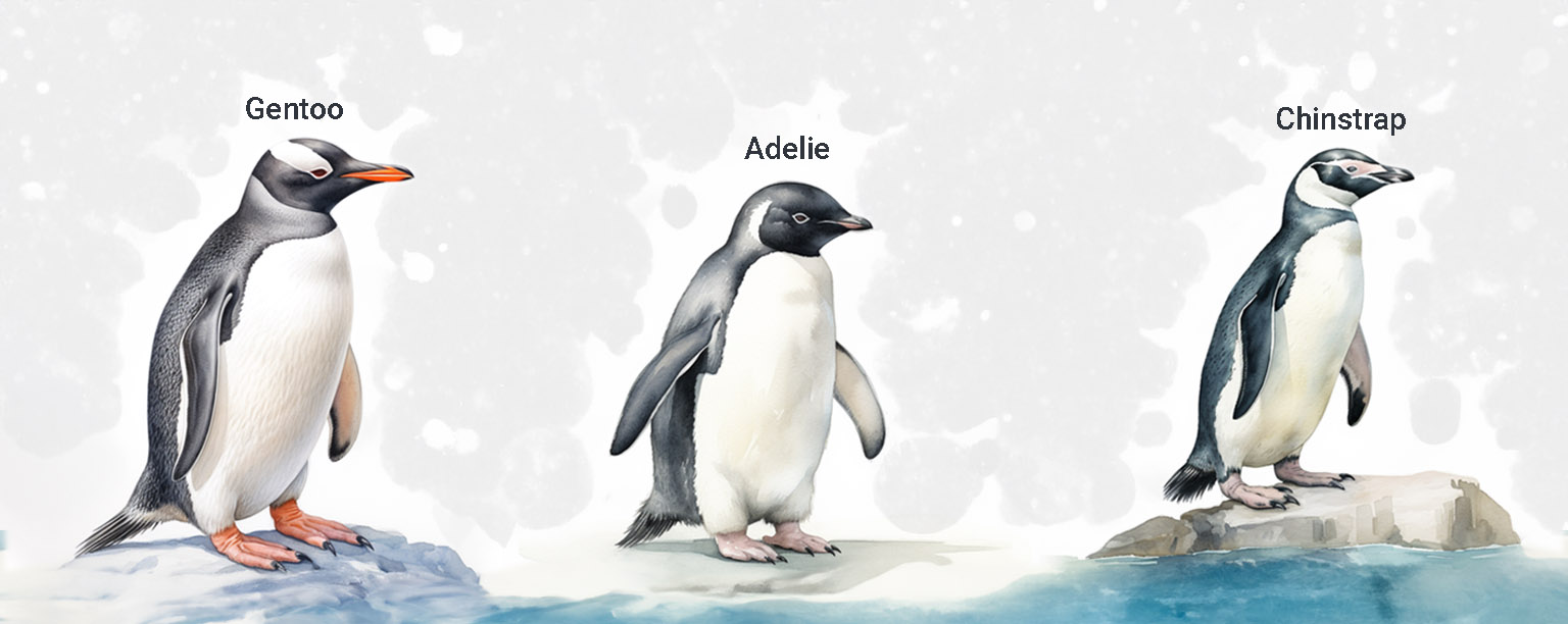
The Palmer Penguins dataset has data from three penguin types from Antarctica’s Palmer islands. These are Adélie, Gentoo, and Chinstrap. It has info like bill lengths and sizes, flipper lengths, and body weight. Check out the “Explore and Experiment” section for more.
Objective
Our goal is to train a machine learning model with this dataset. This model will guess a penguin’s type from its sizes.
Using Maya for Visualization
I added a Maya file with a 3D penguin to make this guide more hands-on. You can change this 3D penguin’s sizes, like its bill length or flipper size. When you do, the trained model will guess its type. This shows how you can use the dataset in 3D.
This guide shows how to mix data science and 3D, showing how to use machine learning in tools like Maya.
How We’ll Proceed
Code Walkthrough
We’ll start with the Python code. I’ll show you the whole script and then explain each part. This will help you see how the machine learning model works, how it learns, and how it guesses.
Diving into Maya
After the code, we’ll look at Maya. We’ll check out the 3D penguin and see what you can change. This part helps you see how the 3D penguin’s sizes match the dataset’s data.
Bringing Code to Scene
Last, we’ll use the Python script in Maya. When you change the 3D penguin’s sizes, you’ll see the model’s guess. This shows how the trained model works in 3D.
By the end, you’ll understand the data science of guessing penguin types and how to show it in 3D in Maya.
Download the Demo Files
You can get all the files for this guide from the link below:
https://github.com/BramVR/penguinFiles/tree/main
Download these files before you move on.
Setting up the Environment
To set up the environment, you need to install the required libraries. Create a file named ‘requirements.txt’ and add the following content to it: If you are using Maya 2022:
werkzeug==2.2.3
tensorflow==2.10.0
scikit-learn==1.0
keras==2.10.0
fonttools==4.38.0
matplotlib==3.5.3
pandas==1.3.5
For Maya 2023+ (with Python 3.9 support):
werkzeug
tensorflow
scikit-learn
keras
fonttools
matplotlib
pandas
protobufNote: Maya 2023 introduced support for Python 3.9. This means that when working with Maya 2023 or later versions, you can use libraries compatible with Python 3.9. In contrast, Maya 2022 uses Python 3.7, which requires specific versions of libraries to ensure compatibility. As a result, with Maya 2023 and onwards, it’s generally safe to install the latest versions of the required libraries, as they are more likely to support Python 3.9.
Open up a new cmd window and navigate to your local Maya 2022 installation folder:
C:\Program Files\Autodesk\Maya2022\binFor Maya 2023+:
C:\Program Files\Autodesk\Maya2023\binNow, run the following command to install the required libraries:
mayapy -m pip install -r path_to_req/requirements.txtCode Walkthrough
Below is the Python code that you will use for the demo. This code should be executed within Maya.
Create the Machine Learning model and saving it
# Import necessary libraries and modules
import pandas as pd
import numpy as np
import tensorflow as tf
from tensorflow.keras.layers import Dense
from tensorflow.keras.utils import to_categorical
from sklearn.preprocessing import StandardScaler
from sklearn.model_selection import train_test_split
from sklearn.metrics import confusion_matrix
import matplotlib.pyplot as plt

# Load the dataset from the specified path
data = pd.read_csv(r'path_to_csv/penguins-clean-all.csv')

# Map species names to numeric values
data['species'] = data['species'].map({'Adelie': 0, 'Gentoo': 1, 'Chinstrap': 2})

# Split the dataset into training (70%) and testing (30%) sets
train_data, test_data = train_test_split(data, test_size=0.3, random_state=42)

# Define the features for the model and standardize them
scaler = StandardScaler()
features = ['bill_length_mm', 'bill_depth_mm', 'flipper_length_mm', 'body_mass_g']
xtrain = scaler.fit_transform(train_data[features])
xtest = scaler.transform(test_data[features])

# Convert the species labels to one-hot encoded format
ytrain_encoded = to_categorical(train_data['species'])
ytest_encoded = to_categorical(test_data['species'])

# Define the neural network model structure
model = tf.keras.Sequential([
    Dense(10, input_shape=(4,), activation="relu"),
    Dense(3, activation="softmax")
])

# Compile the model specifying the optimizer, loss function, and evaluation metric
model.compile(loss='categorical_crossentropy', optimizer=tf.keras.optimizers.SGD(learning_rate=0.01), metrics=['accuracy'])

# Train the model using training data, and validate it using testing data
history = model.fit(xtrain, ytrain_encoded, epochs=50, batch_size=16, validation_data=(xtest, ytest_encoded))

# Plot the model's performance metrics (Accuracy, Loss, Confusion Matrix)
fig, ax = plt.subplots(1, 3, figsize=(18, 6))

# Plot accuracy history for training and validation sets
ax[0].plot(history.history['accuracy'], label='Train')
ax[0].plot(history.history['val_accuracy'], label='Test')
ax[0].set_title('Model Accuracy')
ax[0].set_ylabel('Accuracy')
ax[0].set_xlabel('Epoch')
ax[0].legend()
ax[0].invert_yaxis()

# Plot loss history for training and validation sets
ax[1].plot(history.history['loss'], label='Train')
ax[1].plot(history.history['val_loss'], label='Test')
ax[1].set_title('Model Loss')
ax[1].set_ylabel('Loss')
ax[1].set_xlabel('Epoch')
ax[1].legend()

# Generate and plot the confusion matrix
conf_mat = confusion_matrix(test_data['species'], np.argmax(model.predict(xtest), axis=-1))
cax = ax[2].matshow(conf_mat, cmap='Blues')
fig.colorbar(cax, ax=ax[2])
ax[2].set_title('Confusion Matrix')
ax[2].set_ylabel('Actual')
ax[2].set_xlabel('Predicted')
ax[2].set_xticks([0, 1, 2])
ax[2].set_yticks([0, 1, 2])
ax[2].set_xticklabels(['Adelie', 'Gentoo', 'Chinstrap'])
ax[2].set_yticklabels(['Adelie', 'Gentoo', 'Chinstrap'])
for i in range(conf_mat.shape[0]):
    for j in range(conf_mat.shape[1]):
        ax[2].text(j, i, conf_mat[i, j], ha='center', va='center')

plt.tight_layout()
plt.show()

# Save the scaler
scaler_filename = r'path_to_save_scaler\scaler.save'
joblib.dump(scaler, scaler_filename)
# Save the trained model
model_path = r'path_to_save_model\model.h5'
model.save(model_path)
Code breakdown:
-
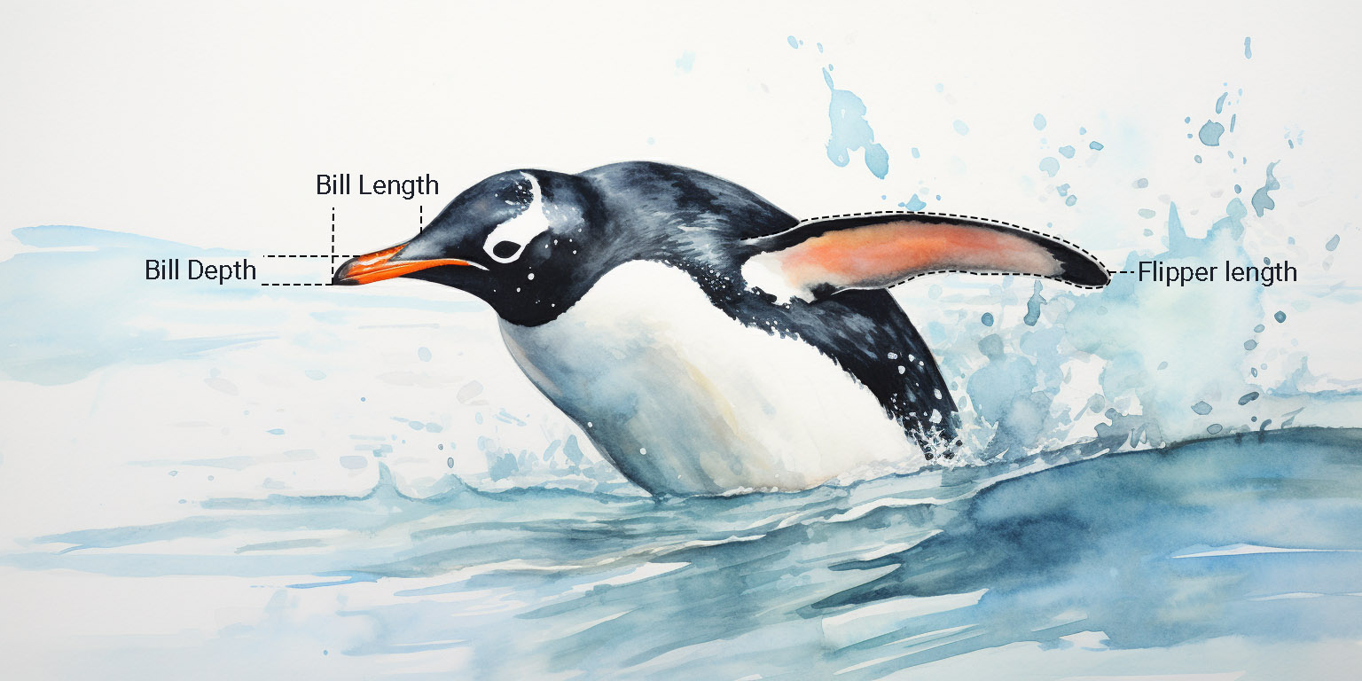
You’re using the Palmer Penguins dataset. It has information on three types of penguins from three islands in Antarctica. The dataset includes details like flipper length and bill depth.
-
Start by loading the dataset so you can work with it.
-
Change the penguin names (like Adelie or Gentoo) from words to numbers. This makes it easier for the computer to understand.
-
Divide the dataset. Use 70% of it to teach the model and 30% to test how well it has learned.
-
Adjust the data so that all the measurements are on a similar scale. The StandardScaler helps with this.
-
Change the penguin species names into a format that the model can use for classification. This is called one-hot encoding.
-
Build the model in steps:
- Start with an input layer for the data.
- Add a hidden layer that does most of the calculations.
- Finish with an output layer that gives the penguin species.
-
Before the model starts learning:
- Set it up (compile it).
- Choose how it should measure how well it’s doing (categorical_crossentropy loss).
- Pick a method for it to improve (SGD optimizer).
-
Let the model learn from the training data. Check how well it’s doing with the test data.
-
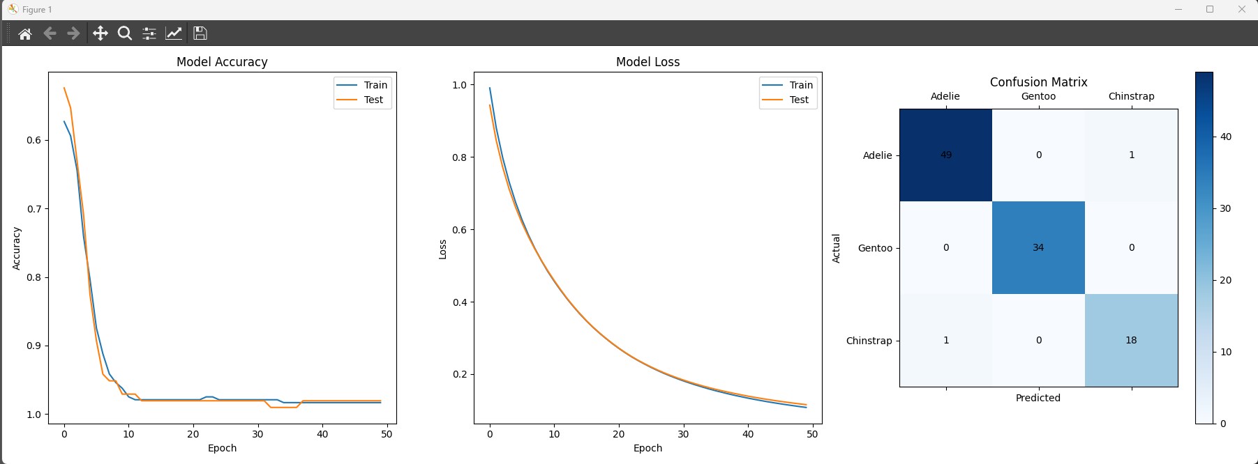
It’s good to see how the model is doing visually:
- Look at a graph of its accuracy.
- See how much it’s getting wrong (loss).
- Use a confusion matrix to see where it’s making mistakes.
-
When you’re done, save your model for later use. Remember to:
- Save the model itself.
- Save the scaler too, so you treat new data the same way as the training data.
Using the Saved Model in Maya
# Import necessary libraries
import numpy as np
import tensorflow as tf
from maya import cmds
from sklearn.preprocessing import StandardScaler
import joblib
import pandas as pd

# Load the saved scaler
scaler_filename = r'path_to_save_scaler/scaler.save'
scaler = joblib.load(scaler_filename)

# Load the saved model
model_path = r'path_to_save_model/model.h5'
model = tf.keras.models.load_model(model_path)

# Fetch custom attributes from Maya
input_data = np.array([cmds.getAttr("main_ctrl.billLength"), cmds.getAttr("main_ctrl.billDepth"),
                       cmds.getAttr("main_ctrl.flipperLength"), cmds.getAttr("main_ctrl.Mass")])

# Convert the ndarray to a DataFrame with feature names
features = ['bill_length_mm', 'bill_depth_mm', 'flipper_length_mm', 'body_mass_g']
input_df = pd.DataFrame([input_data], columns=features)

# Use the loaded scaler to transform the input data
input_data_scaled = scaler.transform(input_df)

# Predict the species using the loaded model
predicted_class = np.argmax(model.predict(input_data_scaled))
predicted_species =['Adelie', 'Gentoo', 'Chinstrap'][predicted_class]
cmds.setAttr("annotationShape1.text", predicted_species, type= "string")
Code Breakdown
-
Start by importing all the necessary libraries. You’ll need numpy for numerical operations, TensorFlow for the neural network, Maya’s `cmds` for interaction with the Maya scene, and `StandardScaler` for data scaling. The `joblib` library is for loading the saved scaler, and `pandas` is used to handle data.
-
Load the previously saved scaler from its path.
-
Next, load the trained model so that predictions can be made without needing to retrain.
-
Fetch the custom attributes from Maya. These are your input features: bill length, bill depth, flipper length, and mass.
-
Convert the gathered attributes to a DataFrame, which is a table-like structure in pandas. This format is necessary for the next step, where we standardize the data.
-
Use the loaded scaler to transform (standardize) your input data, ensuring it’s in the same format as the data used to train the model.
-
Predict the species using the loaded model. The model provides a probability for each species, and `argmax` gives the one with the highest probability.
-
Display the predicted species in Maya by setting the value of a text attribute, in this case, `annotationShape1.text`.
Diving into Maya
Maya Interface
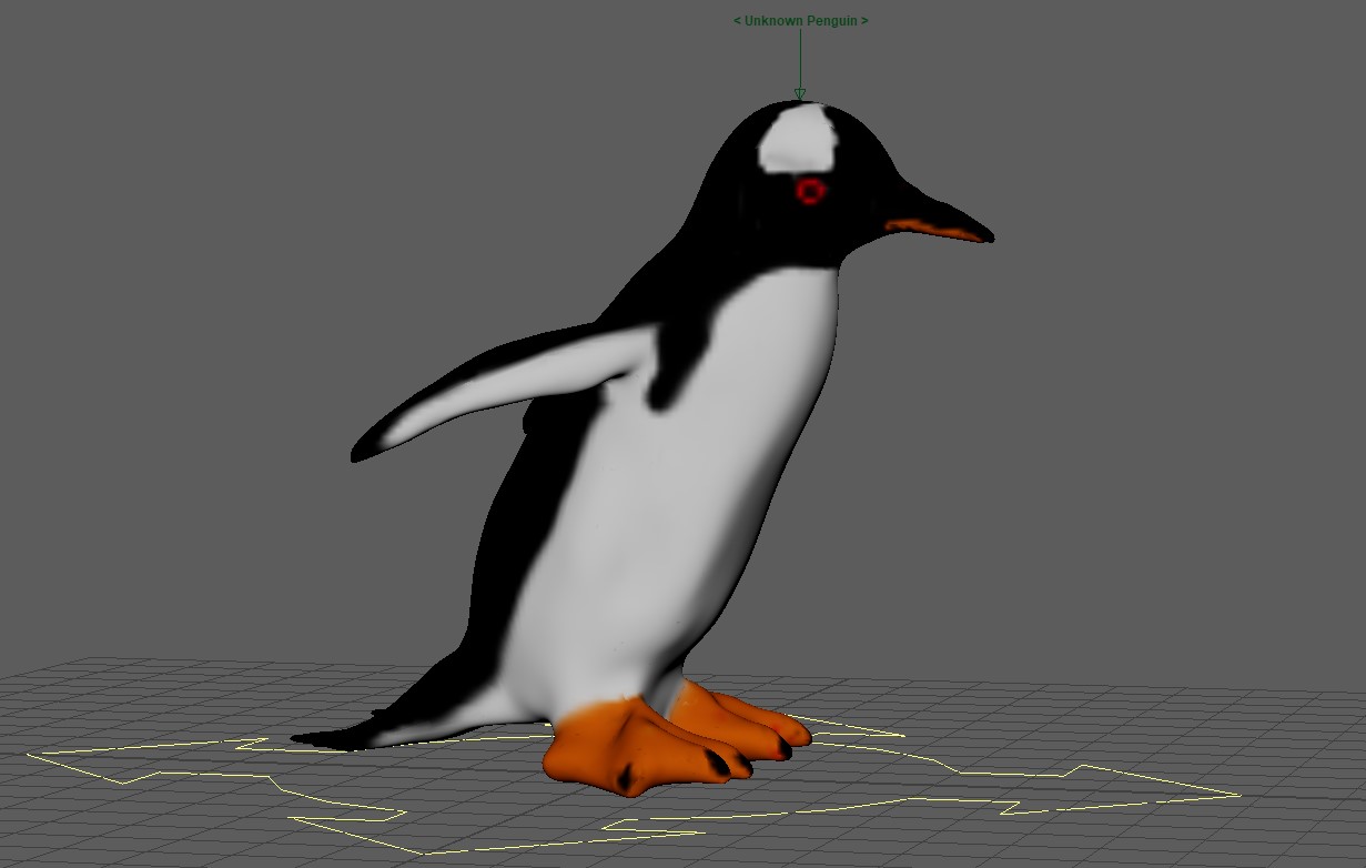
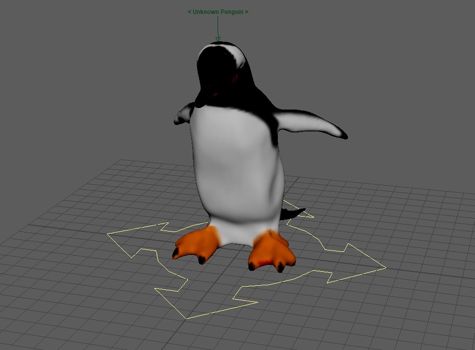
Upon opening the Maya scene, you’ll see a 3D penguin model. This model has adjustable properties linked to our dataset.
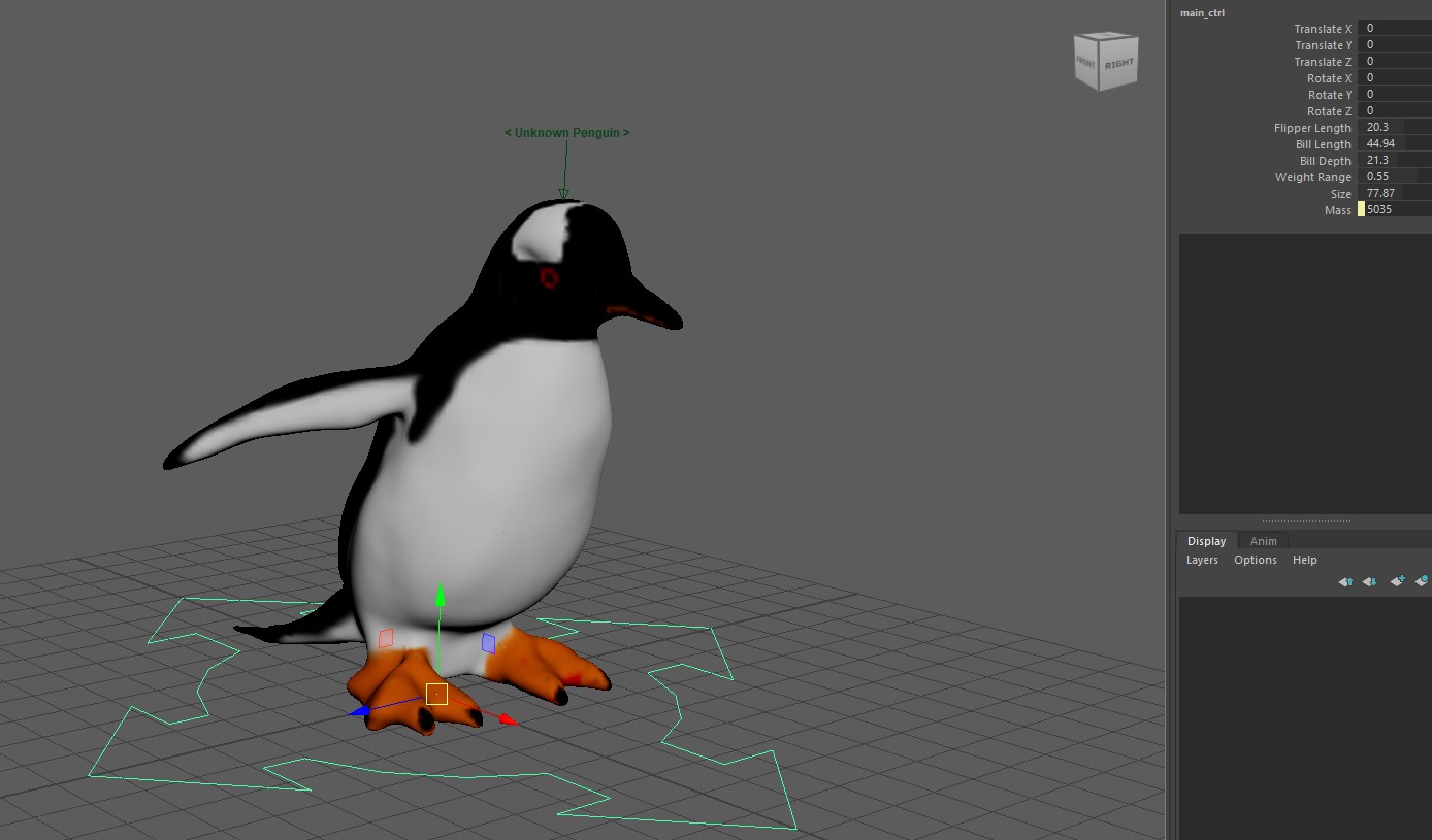
Attributes Overview
You can change these attributes in the rig:
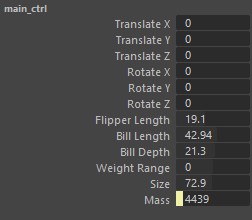
Flipper Length
- It’s about the penguin’s flipper size.
- It matches the `flipper_length_mm` in the dataset.
Bill Length
- This is the penguin’s beak length.
- It matches the `bill_length_mm` in the dataset.
Bill Depth
- This tells how thick the beak is.
- It’s the same as the `bill_depth_mm` in the dataset.
Weight Range
- This goes from -1 to 1.
- -1 is for a thin penguin.
- 0 is the normal look.
- +1 is for a thicker penguin.
Size
- This changes the penguin’s size.
- It goes from 50 to 98, showing different penguin sizes.
Mass (Calculated Attribute)
- This is the penguin’s weight.
- It’s based on the weight and size. When you change those, this changes too.
How Attributes Relate to the Dataset
When you change things in Maya, you’re seeing our dataset in action. Changing these values lets you see different penguin “samples”. This hands-on method makes the data easy to understand in 3D.
Bringing Code to Scene
Prepare Your Scene
Open your Maya scene with the penguin and its changes. We’ll work with this 3D model.
Loading the Dataset
Before we start, make sure you can get to the Palmer Penguins dataset. Check the code to see where it’s looking for this data. This data teaches our model.
Train the Model within Maya
In Maya, use the Python code from the section: “Create the Machine Learning model and saving it”. This code gets the data, gets it ready, sets up the model, and trains it. After it’s done training, it saves the model.
Adjust Penguin Attributes using Maya
After saving the trained model, go to the Maya rig settings. Change the Flipper Length, Bill Length, Bill Depth, Weight Range, Size, and Mass.
Making Predictions using Maya
Use the Python code from the section: “Using the Saved Model in Maya”. When you change the penguin settings in Maya, run the code. It uses the saved model to guess the penguin type.
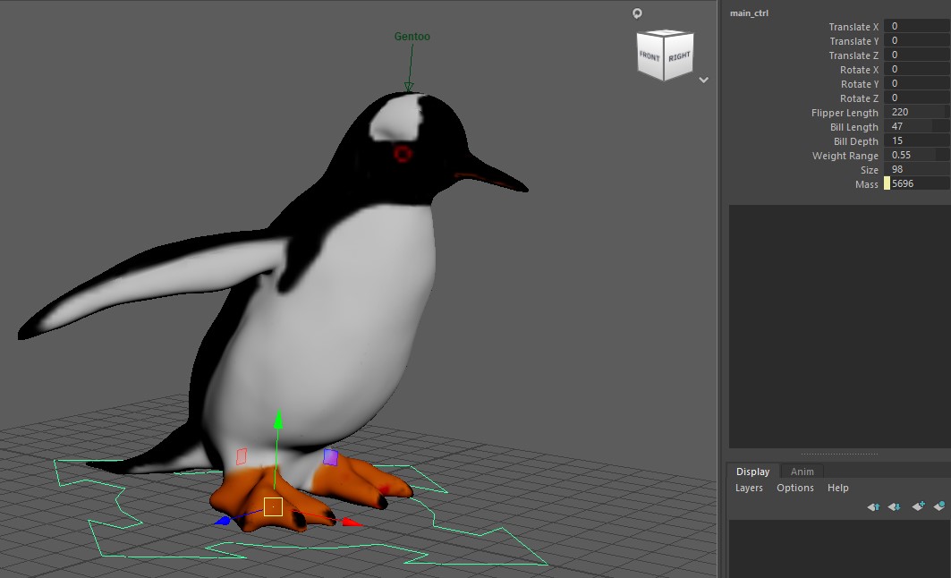
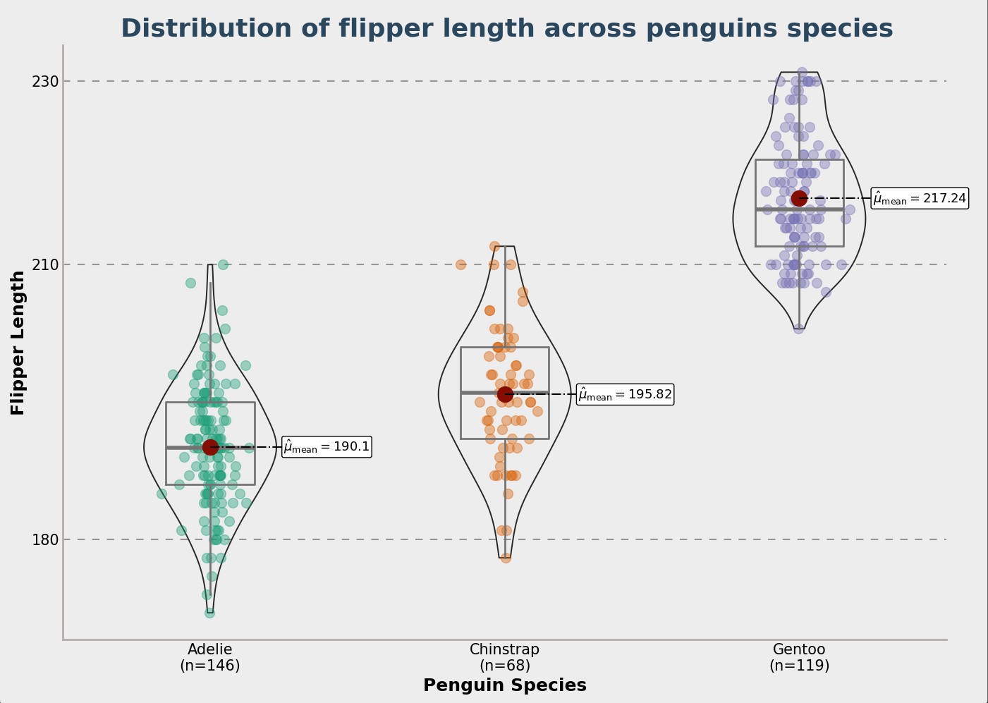
Explore and Experiment
Change the penguin rig settings and see what the model guesses. This helps you understand how the model thinks.
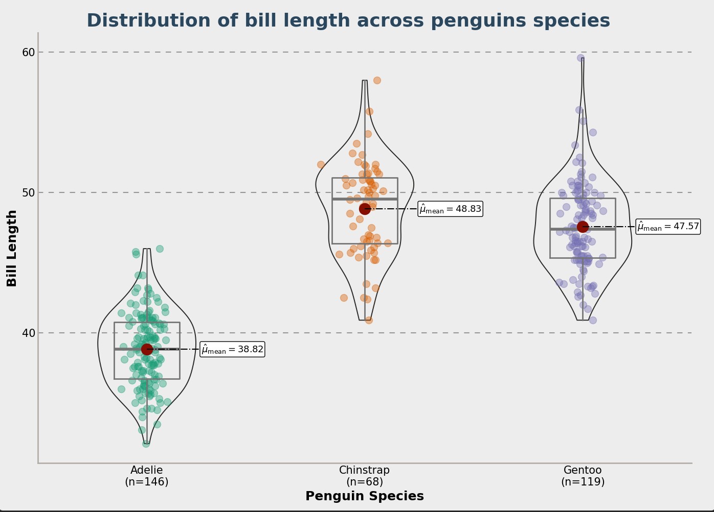
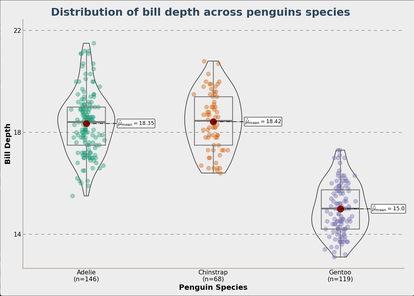
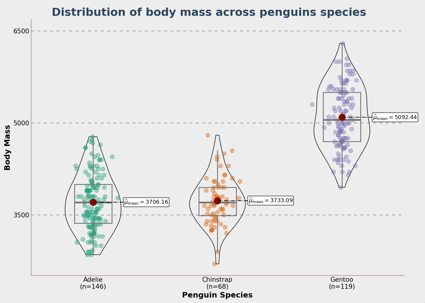
You can see below a few charts that show how the penguin data is spread out. This helps understand the different penguin types.
Conclusion
You’ve now mixed data science and 3D modeling in Maya. You’ve seen how data, like penguin sizes, can be shown in 3D.
By now, you should get both the science of classifying penguins and how to show it in 3D in Maya.